42 excel chart change all data labels at once

Change the position of data labels automatically Click the chart outside of the data labels that you want to change. Click one of the data labels in the series that you want to change. On the Format menu, click Selected Data Labels, and then click the Alignment tab. In the Label position box, click the location you want. previous page start next page. Change the format of data labels in a chart To get there, after adding your data labels, select the data label to format, and then click Chart Elements > Data Labels > More Options. To go to the appropriate area, click one of the four icons ( Fill & Line, Effects, Size & Properties ( Layout & Properties in Outlook or Word), or Label Options) shown here.

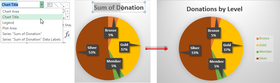
Excel charts: add title, customize chart axis, legend and data labels ... Click anywhere within your Excel chart, then click the Chart Elements button and check the Axis Titles box. If you want to display the title only for one axis, either horizontal or vertical, click the arrow next to Axis Titles and clear one of the boxes: Click the axis title box on the chart, and type the text.

Excel chart change all data labels at once

How to add data labels from different column in an Excel chart? Click any data label to select all data labels, and then click the specified data label to select it only in the chart. 3. Go to the formula bar, type =, select the corresponding cell in the different column, and press the Enter key. See screenshot: 4. Repeat the above 2 - 3 steps to add data labels from the different column for other data points. Excel changes multiple series colors at once - Microsoft Tech Community sub formatseriesthesame() if activechart is nothing then msgbox "select a chart and try again!", vbexclamation goto exitsub end if with activechart dim icolor as long icolor = .seriescollection(2).format.line.forecolor.rgb dim iseries as long for iseries = 3 to .seriescollection.count .seriescollection(iseries).format.line.forecolor.rgb = icolor … How to Change Excel Chart Data Labels to Custom Values? 05/05/2010 · It does chart all 1050 rows of data values in Y at all times. I change the charted data range to 160 or more rows of data (155 to all 1050) and suddenly the labels become random. It will display labels 1, 4 , 6 , 7, 9 , 10, 15, and miss all …

Excel chart change all data labels at once. change all data labels - Excel Help Forum For a new thread (1st post), scroll to Manage Attachments, otherwise scroll down to GO ADVANCED, click, and then scroll down to MANAGE ATTACHMENTS and click again. Now follow the instructions at the top of that screen. New Notice for experts and gurus: Excel chart changing all data labels from value to ... - Stack Overflow By selecting chart then from layout->data labels->more data labels options ->label options ->label contains-> (select)series name, I can only get one series name replacing its respective label values. For more than hundred series stacked in columns i want them all to be changed at once, is there any way out? why it does not change them all at once? Formatting ALL data labels for ALL data series at once Jan 17, 2008. #2. You can pick Show Series for all series of labels at once, if you select the. chart, go to the Chart menu > Chart Options > Data Labels tab. This does all. series at once, not just the ones you've already labeled. You cannot apply other formatting to more than one series of labels at a. time. - Jon. Edit titles or data labels in a chart - support.microsoft.com The first click selects the data labels for the whole data series, and the second click selects the individual data label. Right-click the data label, and then click Format Data Label or Format Data Labels. Click Label Options if it's not selected, and then select the Reset Label Text check box. Top of Page

Format Data Labels in Excel- Instructions - TeachUcomp, Inc. To do this, click the "Format" tab within the "Chart Tools" contextual tab in the Ribbon. Then select the data labels to format from the "Chart Elements" drop-down in the "Current Selection" button group. Then click the "Format Selection" button that appears below the drop-down menu in the same area. excel - Change format of all data labels of a single series at once ... Go straight back to the same data series and right mouse click, and choose add data labels This has worked in Excel 2016. Purely by luck I worked this out saving a great deal of time and frustration. Share answered May 9, 2018 at 13:51 Nic 185 1 9 Add a comment How to change chart axis labels' font color and size in Excel? We can easily change all labels' font color and font size in X axis or Y axis in a chart. Just click to select the axis you will change all labels' font color and size in the chart, and then type a font size into the Font Size box, click the Font color button and specify a font color from the drop down list in the Font group on the Home tab. See below screen shot: Move and Align Chart Titles, Labels, Legends with the ... - Excel Campus Select the element in the chart you want to move (title, data labels, legend, plot area). On the add-in window press the "Move Selected Object with Arrow Keys" button. This is a toggle button and you want to press it down to turn on the arrow keys. Press any of the arrow keys on the keyboard to move the chart element.

Add a DATA LABEL to ONE POINT on a chart in Excel Method — add one data label to a chart line Steps shown in the video above: Click on the chart line to add the data point to. All the data points will be highlighted. Click again on the single point that you want to add a data label to. Right-click and select ' Add data label ' This is the key step! Modify Excel Chart Data Range | CustomGuide Click the Design tab. Click the Select Data button. Select the series you want to change under Legend Entries (Series). Click the Edit button. Type the label you want to use for the series in the Series name field. Click OK. Click OK again. The name is updated in the chart, but the worksheet data remains unchanged. Custom data labels in a chart - Get Digital Help You can easily change data labels in a chart. Select a single data label and enter a reference to a cell in the formula bar. You can also edit data labels, one by one, on the chart. With many data labels, the task becomes quickly boring and time-consuming. But wait, there is a third option using a duplicate series on a secondary axis. Select all Data Labels at once - Microsoft Community The Tab key will move among chart elements. Click on a chart column or bar. Click again so only 1 is selected. Press the Tab key. Each column or bar in the series is selected in turn, then it moves to selecting each data label in the series. Author of "OOXML Hacking - Unlocking Microsoft Office's Secrets", now available

Create Outstanding Pie Charts in Excel | Pryor Learning Solutions

Multiple Time Series in an Excel Chart - Peltier Tech 12/08/2016 · Excel’s line charts use the same data for all series in the chart, or more precisely, for all series on a particular axis. So let’s assign the weekly data to the secondary axis (below left). Excel only gives us the secondary vertical axis, and we really needed the secondary horizontal axis. Using the “+” skittle floating beside the chart (Excel 2013 and later) or the Axis …

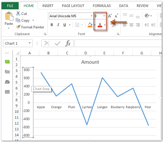
How to change chart axis labels' font color and size in Excel?

Adding rich data labels to charts in Excel 2013 - Microsoft 365 Blog Putting a data label into a shape can add another type of visual emphasis. To add a data label in a shape, select the data point of interest, then right-click it to pull up the context menu. Click Add Data Label, then click Add Data Callout . The result is that your data label will appear in a graphical callout.

Do My Excel Blog: How to design a multiple clustered bar chart series in Excel

Custom Data Labels with Colors and Symbols in Excel Charts - [How To] Step 4: Select the data in column C and hit Ctrl+1 to invoke format cell dialogue box. From left click custom and have your cursor in the type field and follow these steps: Press and Hold ALT key on the keyboard and on the Numpad hit 3 and 0 keys. Let go the ALT key and you will see that upward arrow is inserted.

Adding Data Labels To An Excel Chart | Free Microsoft Excel Tutorials

Edit titles or data labels in a chart - support.microsoft.com You can also place data labels in a standard position relative to their data markers. Depending on the chart type, you can choose from a variety of positioning options. On a chart, do one of the following: To reposition all data labels for an entire data series, click a data label once to select the data series.

Microsoft Tips with Temo!: How to Add Data Labels to an Excel 2010 Chart

How to Change Excel Chart Data Labels to Custom Values? Now, click on any data label. This will select "all" data labels. Now click once again. At this point excel will select only one data label. Go to Formula bar, press = and point to the cell where the data label for that chart data point is defined. Repeat the process for all other data labels, one after another. See the screencast. Points to note:

How-to Use Data Labels from a Range in an Excel Chart - Excel Dashboard Templates

Excel 2010: How to format ALL data point labels SIMULTANEOUSLY Instead of selecting the entire chart, right click one of the data points and select "Format Data Labels". B brianclong Board Regular Joined Apr 11, 2006 Messages 168 May 24, 2011 #3 This still only formats one set of data series labels. Maybe there's a bug? I have Office 64 bit. G gehusi Board Regular Joined Jul 20, 2010 Messages 182 May 24, 2011

Excel Dashboard Templates How-to Put Percentage Labels on Top of a Stacked Column Chart - Excel ...

How to add Axis Labels (X & Y) in Excel & Google Sheets Once you change the title for both axes, the user will now better understand the graph. For example, there is no longer confusion as to whether the revenue is showing in thousands, millions, billions, etc. The axis label has now made it clear that the total revenue is in millions. This is a common example as it helps to make the graph look cleaner.

How to Create a 3-D Cylinder Chart in Your Excel Worksheet - Data Recovery Blog

change format for all data series in chart - Excel Help Forum It might depend on the kind of format change you are trying to do. The only "chart wide" command I can think of is the "change chart type" command. So, if you have a scatter chart with markers and no lines and you want to add lines to each data series, you could go into the change chart type, and change to a scatter with markers and lines.

Fixing Your Excel Chart When the Multi-Level Category Label Option is Missing. - Excel Dashboard ...

Add data labels to your Excel bubble charts | TechRepublic Right-click the data series and select Add Data Labels. Right-click one of the labels and select Format Data Labels. Select Y Value and Center. Move any labels that overlap. Select the data labels ...

How to Make Charts and Graphs in Excel | Smartsheet

Change the labels in an Excel data series | TechRepublic Click the Chart Wizard button in the Standard toolbar. Click Next. Click the Series tab. Click the Window Shade button in the Category (X) Axis. Labels box. Select B3:D3 to select the labels in ...

Excel Dashboard Templates Fixing Your Excel Chart When the Multi-Level Category Label Option is ...

Insert a chart from an Excel spreadsheet into Word Keep Source Formatting & Link Data. Keeps the Excel theme. Keeps the chart linked to the original workbook. To update the chart automatically, change the data in the original workbook. You also can select Chart Tools> Design > Refresh Data. Picture. Becomes a picture. You can’t update the data or edit the chart, but you can adjust the chart ...

Excel Dashboard Templates How-to Put Percentage Labels on Top of a Stacked Column Chart - Excel ...

How to Make a Bar Chart in Microsoft Excel 10/07/2020 · You can make many formatting changes to your chart, should you wish to. You can change the color and style of your chart, change the chart title, as well as add or edit axis labels on both sides. It’s also possible to add trendlines to your Excel chart, allowing you to see greater patterns (trends) in your data. This would be especially ...

How to Create a Column Chart in Excel | onsite-training.com

How to add or move data labels in Excel chart? - ExtendOffice In Excel 2013 or 2016. 1. Click the chart to show the Chart Elements button . 2. Then click the Chart Elements, and check Data Labels, then you can click the arrow to choose an option about the data labels in the sub menu. See screenshot: In Excel 2010 or 2007. 1. click on the chart to show the Layout tab in the Chart Tools group. See ...

30 How To Add Label To Excel Chart - Labels Database 2020

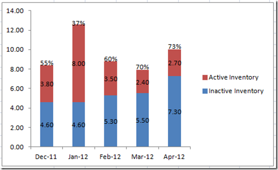
How to Add Total Data Labels to the Excel Stacked Bar Chart Step 4: Right click your new line chart and select "Add Data Labels" Step 5: Right click your new data labels and format them so that their label position is "Above"; also make the labels bold and increase the font size. Step 6: Right click the line, select "Format Data Series"; in the Line Color menu, select "No line" Step 7 ...

Show Trend Arrows in Excel Chart Data Labels

How to Create a Timeline Chart in Excel – Automate Excel In order to polish up the timeline chart, you can now add another set of data labels to track the progress made on each task at hand. Right-click on any of the columns representing Series “Hours Spent” and select “Add Data Labels.” Once there, right-click on any of the data labels and open the Format Data Labels task pane. Then, insert ...

How to Change Excel Chart Data Labels to Custom Values?

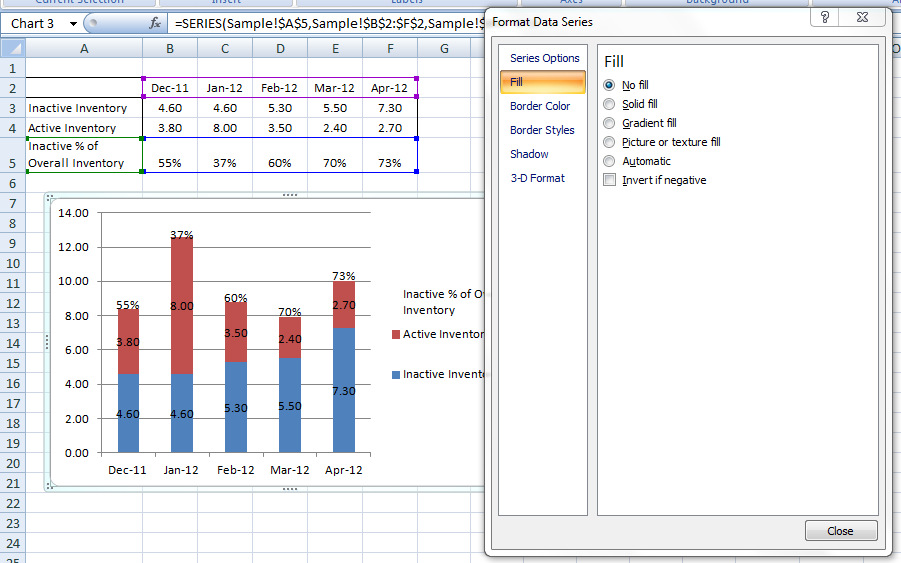
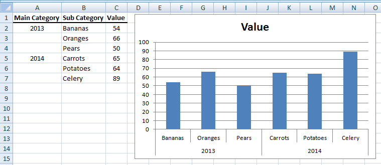
Create a multi-level category chart in Excel - ExtendOffice 2. Select the data range, click Insert > Insert Column or Bar Chart > Clustered Bar.. 3. Drag the chart border to enlarge the chart area. See the below demo. 4. Right click the bar and select Format Data Series from the right-clicking menu to open the Format Data Series pane.. Tips: You can also double click any of the bars to open the Format Data Series pane.

Share :